Pulse shapes¶

import matplotlib.pyplot as plt
import numpy as np
import scipy.signal

import sdr

%config InlineBackend.print_figure_kwargs = {"facecolor" : "w"}
%matplotlib inline
# %matplotlib widget

sdr.plot.use_style()

span = 8  # Length of the pulse shape in symbols
sps = 10  # Samples per symbol

Create a rectangular pulse shape for reference.

rect = np.zeros(sps * span + 1)
rect[rect.size // 2 - sps // 2 : rect.size // 2 + sps // 2] = 1 / np.sqrt(sps)

Raised cosine¶

Create three raised cosine pulses with different excess bandwidths. This is achieved using the sdr.raised_cosine() function.

rc_0p1 = sdr.raised_cosine(0.1, span, sps)
rc_0p5 = sdr.raised_cosine(0.5, span, sps)
rc_0p9 = sdr.raised_cosine(0.9, span, sps)

plt.figure()
sdr.plot.impulse_response(rect, color="k", linestyle=":", label="Rectangular")
sdr.plot.impulse_response(rc_0p1, label=r"$\alpha = 0.1$")
sdr.plot.impulse_response(rc_0p5, label=r"$\alpha = 0.5$")
sdr.plot.impulse_response(rc_0p9, label=r"$\alpha = 0.9$")
plt.show()

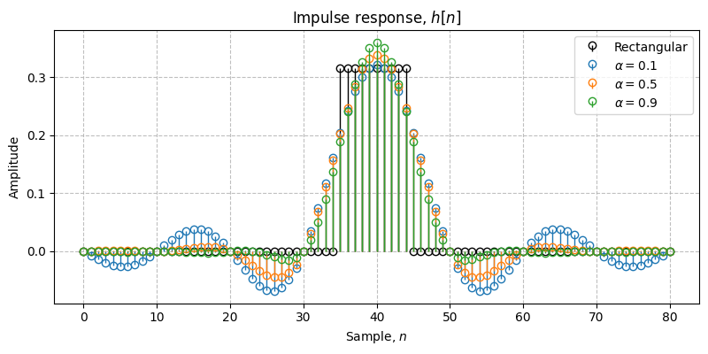
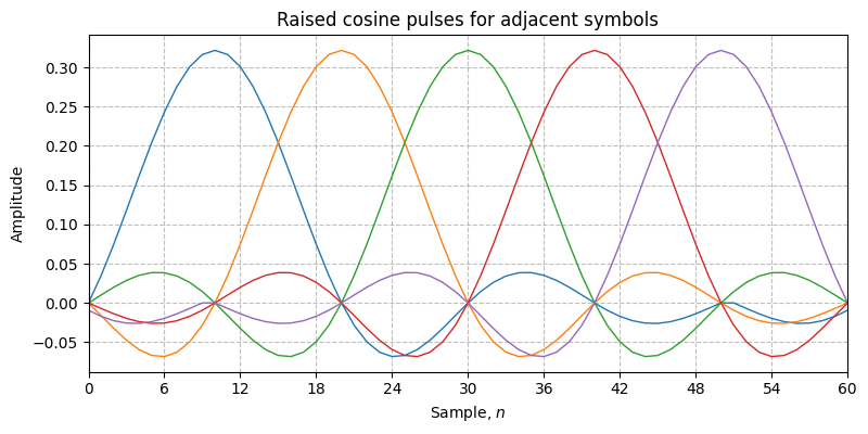
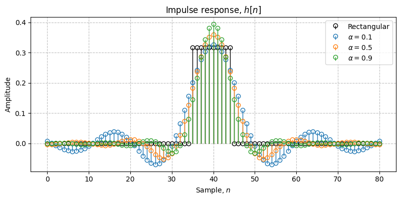
../../_images/7f9d4459b7066f2367973edac192af352d2af3ac68cd5a6ac31f0f3208243a8c.png

The raised cosine filter is a Nyquist filter. This means that the impulse response \(h[n]\) is zero at adjacent symbols. Specifically, \(h[n] = 0\) for \(n = \pm k\ T_s / T_{sym}\)

plt.figure()
sdr.plot.time_domain(np.roll(rc_0p1, -3 * sps))
sdr.plot.time_domain(np.roll(rc_0p1, -2 * sps))
sdr.plot.time_domain(np.roll(rc_0p1, -1 * sps))
sdr.plot.time_domain(np.roll(rc_0p1, 0 * sps))
sdr.plot.time_domain(np.roll(rc_0p1, 1 * sps))
plt.xlim(0, 60)
plt.title("Raised cosine pulses for adjacent symbols")
plt.show()

../../_images/2d4daeec71c708e383e126bdb5bcbe60b2e86804c2a6d0193df933528bf299fd.png

plt.figure()
sdr.plot.magnitude_response(rect, sample_rate=sps, color="k", linestyle=":", label="Rectangular")
sdr.plot.magnitude_response(rc_0p1, sample_rate=sps, label=r"$\alpha = 0.1$")
sdr.plot.magnitude_response(rc_0p5, sample_rate=sps, label=r"$\alpha = 0.5$")
sdr.plot.magnitude_response(rc_0p9, sample_rate=sps, label=r"$\alpha = 0.9$")
plt.xlabel("Normalized frequency, $f/f_{sym}$")
plt.show()

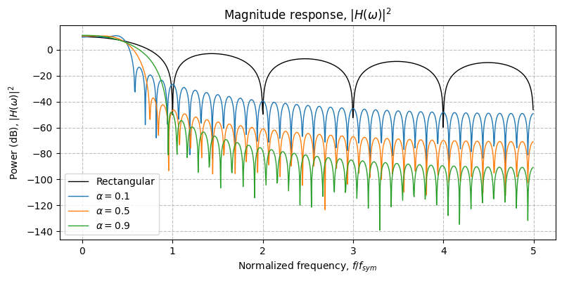
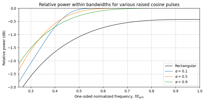
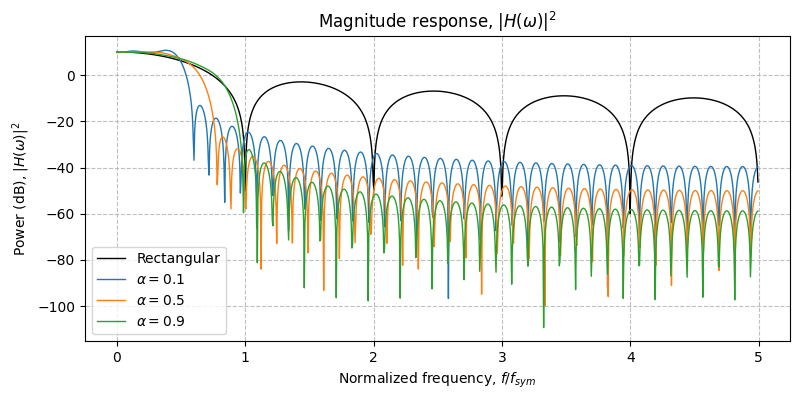
../../_images/4f8fa03852914a718caa577566b8f9f8a1b7634b27f05c3fd744488cac5d494e.png

Notice the raised cosine pulse with excess bandwidth \(\alpha = 0.1\) has a total bandwidth of nearly \(f_{sym}\). Compare this to \(\alpha = 0.9\), which has a null-to-null bandwidth of nearly \(2 f_{sym}\).

While small \(\alpha\) produces a filter with smaller bandwidth, its side lobes are much higher.

# Compute the one-sided power spectral density of the pulses
w, H_rect = scipy.signal.freqz(rect, 1, worN=1024, whole=False, fs=sps)
w, H_rc_0p1 = scipy.signal.freqz(rc_0p1, 1, worN=1024, whole=False, fs=sps)
w, H_rc_0p5 = scipy.signal.freqz(rc_0p5, 1, worN=1024, whole=False, fs=sps)
w, H_rc_0p9 = scipy.signal.freqz(rc_0p9, 1, worN=1024, whole=False, fs=sps)

# Compute the relative power in the main lobe of the pulses
P_rect = sdr.db(np.cumsum(np.abs(H_rect) ** 2) / np.sum(np.abs(H_rect) ** 2))
P_rc_0p1 = sdr.db(np.cumsum(np.abs(H_rc_0p1) ** 2) / np.sum(np.abs(H_rc_0p1) ** 2))
P_rc_0p5 = sdr.db(np.cumsum(np.abs(H_rc_0p5) ** 2) / np.sum(np.abs(H_rc_0p5) ** 2))
P_rc_0p9 = sdr.db(np.cumsum(np.abs(H_rc_0p9) ** 2) / np.sum(np.abs(H_rc_0p9) ** 2))

plt.figure()
plt.plot(w, P_rect, color="k", linestyle=":", label="Rectangular")
plt.plot(w, P_rc_0p1, label=r"$\alpha = 0.1$")
plt.plot(w, P_rc_0p5, label=r"$\alpha = 0.5$")
plt.plot(w, P_rc_0p9, label=r"$\alpha = 0.9$")
plt.legend()
plt.xlim(0.25, 1)
plt.ylim(-3, 0)
plt.xlabel("One-sided normalized frequency, $f/f_{sym}$")
plt.ylabel("Relative power (dB)")
plt.title("Relative power within bandwidths for various raised cosine pulses")
plt.show()

../../_images/49684a4ffa95218ef17340daea8c2536b55a1c7eb077a55d1c4972ac940f165f.png

Square-root raised cosine¶

Create three square-root raised cosine pulses with different excess bandwidths. This is achieved using the sdr.root_raised_cosine() function.

srrc_0p1 = sdr.root_raised_cosine(0.1, span, sps)
srrc_0p5 = sdr.root_raised_cosine(0.5, span, sps)
srrc_0p9 = sdr.root_raised_cosine(0.9, span, sps)

plt.figure()
sdr.plot.impulse_response(rect, color="k", linestyle=":", label="Rectangular")
sdr.plot.impulse_response(srrc_0p1, label=r"$\alpha = 0.1$")
sdr.plot.impulse_response(srrc_0p5, label=r"$\alpha = 0.5$")
sdr.plot.impulse_response(srrc_0p9, label=r"$\alpha = 0.9$")
plt.show()

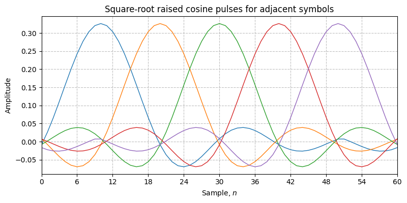
../../_images/a361fa0f6730d19bc1fc87175386bc043e123622be00f0ae9af0354b20ef1c9f.png

The square-root raised cosine filter is not a Nyquist filter. Therefore, the impulse response \(h[n]\) is not zero at adjacent symbols.

plt.figure()
sdr.plot.time_domain(np.roll(srrc_0p1, -3 * sps))
sdr.plot.time_domain(np.roll(srrc_0p1, -2 * sps))
sdr.plot.time_domain(np.roll(srrc_0p1, -1 * sps))
sdr.plot.time_domain(np.roll(srrc_0p1, 0 * sps))
sdr.plot.time_domain(np.roll(srrc_0p1, 1 * sps))
plt.xlim(0, 60)
plt.title("Square-root raised cosine pulses for adjacent symbols")
plt.show()

../../_images/1266640517e8e9b23a74e6173dbffa20de7a7844024ca565c97d00b8158ff53c.png

plt.figure()
sdr.plot.magnitude_response(rect, sample_rate=sps, color="k", linestyle=":", label="Rectangular")
sdr.plot.magnitude_response(srrc_0p1, sample_rate=sps, label=r"$\alpha = 0.1$")
sdr.plot.magnitude_response(srrc_0p5, sample_rate=sps, label=r"$\alpha = 0.5$")
sdr.plot.magnitude_response(srrc_0p9, sample_rate=sps, label=r"$\alpha = 0.9$")
plt.xlabel("Normalized frequency, $f/f_{sym}$")
plt.show()

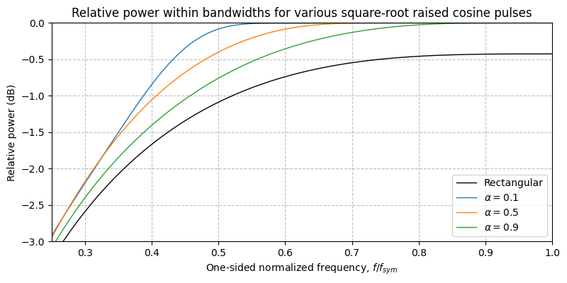
../../_images/89947c9a05bd1fe0c27a73c91537637448322d305624f93ac522266211bbb489.png

While the bandwidths of the square-root raised cosine filter are similar to the raised cosine filter, the side lobes are significantly higher. This is due to this filter not being a Nyquist filter.

# Compute the one-sided power spectral density of the pulses
w, H_rect = scipy.signal.freqz(rect, 1, worN=1024, whole=False, fs=sps)
w, H_srrc_0p1 = scipy.signal.freqz(srrc_0p1, 1, worN=1024, whole=False, fs=sps)
w, H_srrc_0p5 = scipy.signal.freqz(srrc_0p5, 1, worN=1024, whole=False, fs=sps)
w, H_srrc_0p9 = scipy.signal.freqz(srrc_0p9, 1, worN=1024, whole=False, fs=sps)

# Compute the relative power in the main lobe of the pulses
P_rect = sdr.db(np.cumsum(np.abs(H_rect) ** 2) / np.sum(np.abs(H_rect) ** 2))
P_srrc_0p1 = sdr.db(np.cumsum(np.abs(H_srrc_0p1) ** 2) / np.sum(np.abs(H_srrc_0p1) ** 2))
P_srrc_0p5 = sdr.db(np.cumsum(np.abs(H_srrc_0p5) ** 2) / np.sum(np.abs(H_srrc_0p5) ** 2))
P_srrc_0p9 = sdr.db(np.cumsum(np.abs(H_srrc_0p9) ** 2) / np.sum(np.abs(H_srrc_0p9) ** 2))

plt.figure()
plt.plot(w, P_rect, color="k", linestyle=":", label="Rectangular")
plt.plot(w, P_srrc_0p1, label=r"$\alpha = 0.1$")
plt.plot(w, P_srrc_0p5, label=r"$\alpha = 0.5$")
plt.plot(w, P_srrc_0p9, label=r"$\alpha = 0.9$")
plt.legend()
plt.xlim(0.25, 1)
plt.ylim(-3, 0)
plt.xlabel("One-sided normalized frequency, $f/f_{sym}$")
plt.ylabel("Relative power (dB)")
plt.title("Relative power within bandwidths for various square-root raised cosine pulses")
plt.show()

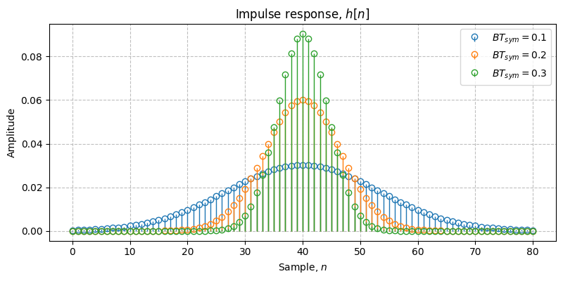
../../_images/17a3c7468738c449a79002b3a473137ad5a19520292679667b9104b8bd2b0f76.png

Gaussian¶

Create three raised Gaussian pulses with different time-bandwidth products. This is achieved using the sdr.gaussian() function.

gauss_0p1 = sdr.gaussian(0.1, span, sps)
gauss_0p2 = sdr.gaussian(0.2, span, sps)
gauss_0p3 = sdr.gaussian(0.3, span, sps)

plt.figure()
sdr.plot.impulse_response(gauss_0p1, label=r"$B T_{sym} = 0.1$")
sdr.plot.impulse_response(gauss_0p2, label=r"$B T_{sym} = 0.2$")
sdr.plot.impulse_response(gauss_0p3, label=r"$B T_{sym} = 0.3$")
plt.show()

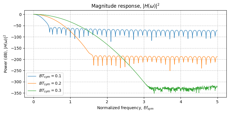
../../_images/0a419c0f57c4b2f54105da7e1cae56c599bb529bbdec88784818f62c5be67a44.png

plt.figure()
sdr.plot.magnitude_response(gauss_0p1, sample_rate=sps, label=r"$B T_{sym} = 0.1$")
sdr.plot.magnitude_response(gauss_0p2, sample_rate=sps, label=r"$B T_{sym} = 0.2$")
sdr.plot.magnitude_response(gauss_0p3, sample_rate=sps, label=r"$B T_{sym} = 0.3$")
plt.xlabel("Normalized frequency, $f/f_{sym}$")
plt.show()

/home/matt/repos/sdr/src/sdr/plot/_filter.py:356: RuntimeWarning: divide by zero encountered in log10
  H = 10 * np.log10(np.abs(H) ** 2)

../../_images/50e243aca56934dd3b9e661a6a2e880f0483d9210c5c21773f3c95deea5edd6b.png

Last update: Feb 24, 2024